This article illustrates what the work of modeling a problem for constraint #optimization entails.

A #problem with a vague description

Unless you’ve been living under a rock, you are aware that the COVID19 pandemic happened and is still ongoing. One thing that has become common at least in rich countries is the frequent tests we need to perform to validate whether a person is infected or not. A variety of test technologies have different characteristics, some tests can be done at home (rapid anti-genic tests). Whereas PCR tests need a specific person to carry the sample then the samples are sent to a laboratory that processes the PCR check.

Now let’s say there is some imbalance between PCR-check laboratories and some tests sites. A question that may arise is: how do we best allocate samples from various sampling locations (e.g., pharmacies) to laboratories? There is some delay in sending tests to laboratories, and also there is a maximum delay to wait for a sample (otherwise the sample deteriorates and can no longer provide good material for the test). What do we do for a day, over a week?

An off-the-shelf model

Before using a modeling approach solver, it’s always good to verify whether the problem has an easy-to-recognize shape. This instance looks like an max-flow problem where testing locations are sources and laboratories are samples: indeed maximizing the number of samples that go through testing is a way to minize those which are thrown out.

The following example shows a possible max-flow #model to this problem. On the left you have a fictional demand node and on the right a fictional processed node. The from arrows are capacities which corresponds to the demand at each sample-collection location. The symmetric side of processing- capacities are to arrows. The center arrows with ? are the attribution matrix. We could force some capacities to zero to say a sample-location is too far from a certain site, or leave them infinite to express that any amount of samples can be sent.

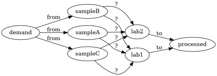
Running max-flow on this graph would determine how to maximize the number of processed samples. And the actual-values achieved the ? arrows correspond to a best assignment.

This is all good but in real-life we need to consider multiple days and other constraints. The iterated aspects may be annoying to model but somewhat manageable. For instance, we could add staged sources and sinks where some capacity connects a laboratory at two time intervals (this way leftovers can be post-poned as additional inputs). In the following picture, we add a suffix _0 and _1 to represent the different stages. Thus an arrow lab1_0 -> lab1_1 represents leftovers at lab1 from the first staged processed in the second stage. We could view these arrows across stages as a degenerate form of sending samples between two different places in the time dimension.

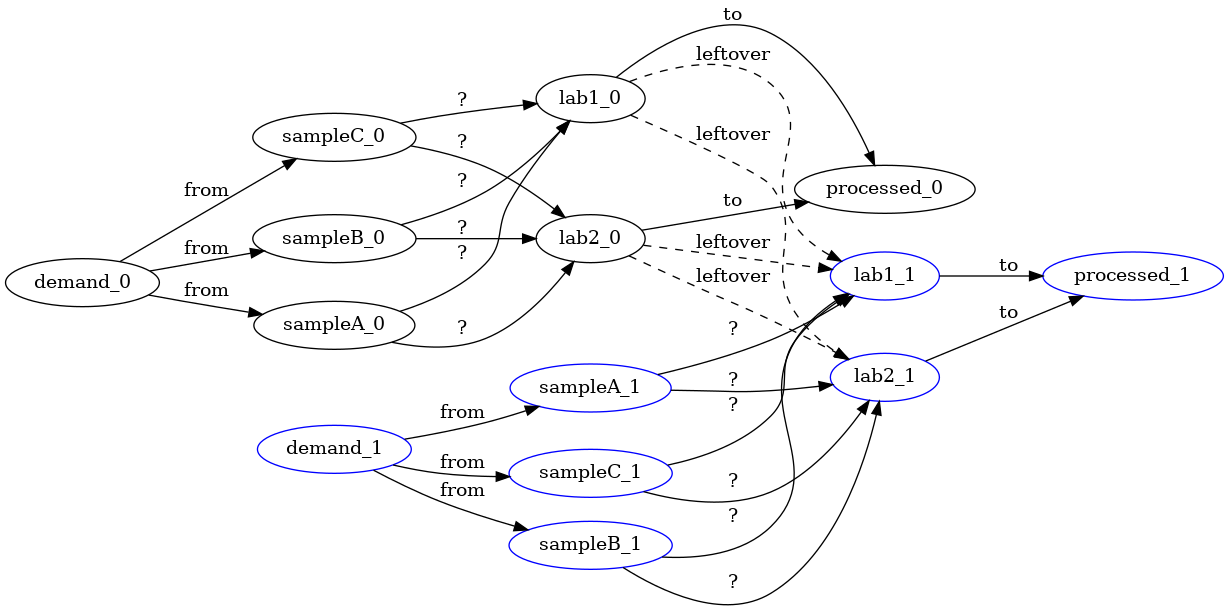
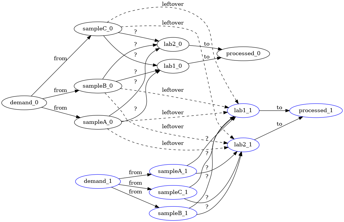
Such a model starts to be slightly more cumbersome than the previous one, and also is wrong because we do not properly model the deadline component. For instance, with many stages we could have a long chain of leftover samples until all samples are processed, irrespective from how old the samples are. Instead of having leftovers from labs to labs at future time-steps, we rather need the leftover arrows to go from sampling location to lab at future time-steps. Correcting for this fact we get the following schema:

This model now seems correct and useful. However, in real-world setups we often refine models as new constraints are discovered or as new decisions are required. For instance, one behavior that would significantly alter the model would be to limit sampling sites to send samples to at most two labs. We may have to scrap our solution because the max-flow algorithm is not “cut” to make choices between alternatives (what we need is a form of knapsack at each sample-collection location). Such situations are common, and they correspond to situations where constraint-programming modeling shines. Constraint programming will let you trade generality for performance (i.e., we expect a slow down by using a more-general approach). Other situations where the adaptability of constraint-programming is useful is to probe what happens when a constraint actually turns-out to be a secondary goal (i.e., we relax a hard constraint into a soft-constraint and pretend we are geniuses).

Enough introduction, let’s see how we could formulate the problem in a constraint-programming language (using MiniZinc as usual on this blog).

A constraint-programming model

Remember that to model a constraint-programming problem we need to formulate what are inputs, decisions, and constraints. We also need some form of objective.

high-level model

We will assume that we have some time-based model of the demand in number of tests. We also assume that we know the labs capacities (this is no different from our introductory model).

In our case, a good starting point would be:

inputs

• demand for samples from sample-collection locations
• PCR lab capacities
• some measure of the time it takes to send samples from one testing-site to a lab
• the duration for which a sample is valid

decisions

• some assignment from testing-sites to labs

constraints

• samples must be processed within their lifetime or will be wasted
• labs total work cannot overshoot their capacity
• some form of conservation law to say that samples are either tested in time or thrown away

objective

• minimize the number of samples thrown away otherwise you can always assign zero from any testing-site to any lab

formalized in MiniZinc

The core of the model would be something as follows:

int: nLab;
int: nZone;
int: nTime;
int: sample_lifetime;

set of int: LAB = 1..nLab;
set of int: ZONE = 1..nZone;
set of int: TIME = 1..nTime;
set of int: DELAY = 0..sample_lifetime;

% demand of samples produced by zones
array[ZONE,TIME] of int: demand;
% capacity of labs to process samples, may vary with time to model things like week-ends
array[LAB] of int: capacity;
% transit represents a delay from one zone to some lab
array[ZONE,LAB] of int: transit;


% decisions about routing samples: dispatching and dropping samples
int: maxAttr = sum(z in ZONE, t in TIME)(demand[z,t]);
array[ZONE,LAB,TIME,DELAY] of var 0..maxAttr: dispatch;
array[ZONE,TIME] of var 0..maxAttr: dropped;

Which introduces the inputs and the key decisions. We name ZONE the set of sampling-locations because we could aggregate locations into zones beforehand, but also because we I found it hard to juggle with LAB and LOC all the time in my mind.

More importantly, we refined the decision to explicitly add a DELAY component to the dispatch-ed amount from a given ZONE to a given LAB at a given TIME. This delay corresponds to the dashed arrows we introduced in the max-flow model before. This extra breakdown is not especially surprising because we need to model the same “allowed physical behavior” whatever modeling technique we use. That said, in this model we went a bit further and we have broken down the total delay into two components: transit times (which are imposed by the transit matrix) and queuing time (i.e., if a lab is busy one day but as spare capacity the next day we can backlog). The framing is very similar but are being a bit more explicit which chunk of the delay is forced upon us versus what chunk of the delay is a proper decision: this break down is important if you were to iterate on the model, or decide to increase capacity.

We also have a separate explicit dropped decision, for all the samples that we cannot process. This decision is new compared to the max-flow model because in the max-flow model dropped quantities are implicit: dropped quantities correspond to amount of demand flow under the attributed capacity. In constraint-programming it is somewhat required to be explicit otherwise the solver will typically find an “uninteresting” solution (e.g., deciding that we drop everything implicitly because we have no way to express the conservation law).

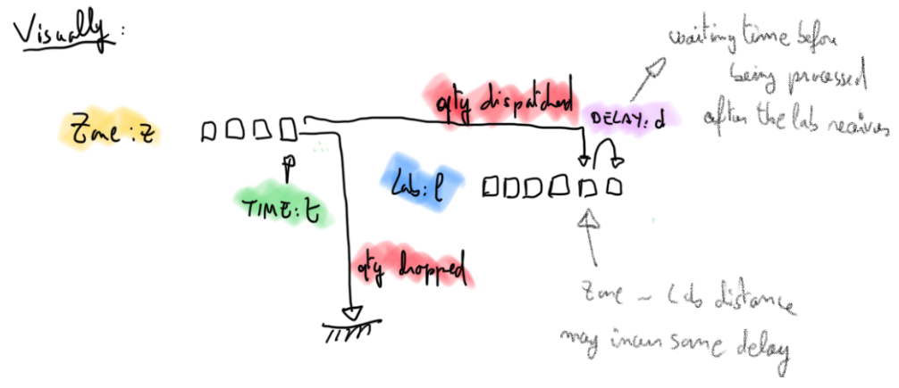
Visually I represented this model as follows, in case it helps (demand at different times for a given zone are on the left, load for a given lab is the right).

We still need to link everything with constraints and write the objective function.

conservation law

The conservation-law is not too complicated: at any given TIME, the demand is partitioned in two sets: dropped quantities and dispatched quantities.

% must dispatch all demand
constraint forall(z in ZONE, t in TIME)
  (demand[z,t] - dropped[z,t] = sum(l in LAB, d in DELAY)( dispatch[z,l,t,d] ));

Such conservation laws are often “hidden” behind inequalities. In this case I initially had a inequality saying that the dispatched amount had to be below the demand, it took me some time to realize that what is leftover deserves a concept in its own. Then, the conservation law appeared and it became easier to reason and debug with this extra ‘dropped’ variable.

samples must reach a lab and be processed within their lifetime

Here we are using some implication connective that says that if the transit time and the considered queuing delay exceeds the sample lifetime, then the dispatched amount for this zone, lab, and delay has to be zero.

% cannot delay (including transit time) past sample_lifetime
constraint forall(z in ZONE, l in LAB, t in TIME, d in DELAY)
  ((transit[z,l] + d > sample_lifetime) -> dispatch[z,l,t,d] = 0);

This formal statement is worth reading at a slow pace because the formalism is not really a natural way of thinking. What makes such statements hard to parse is that we initially said that we want samples to be processed within their lifetime (i.e., we want a desired outcome to happen) whereas the statement speaks about preventing dispatching (i.e., we prevent the inverse of the desired outcome). I do not claim that it is impossible to reverse the logic, but I found no trivial ways to do so without introducing new variables.

Combined with the conservation law, this constraint will force undispatcheable quantities to move to the dropped quantity.

load versus capacity at LAB

We need some way to prevent LABs overload. For this we need a definition of load of a LAB at a given time. This load consists of the dispatched amounts (including transit costs and backlog-delays).

% helper: workload processed by a lab at a given time (includes delayed dispatches)
array[LAB,TIME] of var int: load;
constraint forall(l in LAB, t_load in TIME)
 ( load[l,t_load] = sum(t_route in t_load-sample_lifetime..t_load where t_route > 0, z in ZONE)
                       (dispatch[z,l,t_route,t_load-t_route])
 );

It takes some work to sum all the right terms, but once we have the load at a given time, the constraint becomes trivial.

% cannot overload labs
constraint forall(l in LAB, t in TIME)
  (capacity[l] >= load[l,t]);

objective: no waste

This probably is the easiest part of the work. We sum the total dropped amounts and minimize this.

var int: total_drop = sum(array1d(dropped));

solve minimize total_drop;

Overall, this objective combined with the conservation law gives some intuition about what a performing heuristic could look like: starting by dispatching zero we try to attribute fill labs with from closest zones in total delay. Fortunately, we do not need to write a heuristic and can just run our MiniZinc model.

Running the model

You will find my model, some example data and even some synthetic-data generator written with a simple Ruby script at one of my GitHub repos .

The final model has one modification (see below) but also a slightly different output format than you get by default with MiniZinc (hopefully it’s more readable).

An example simple input that allows to understand what happens is a data file like the following:

nLab = 3;
nZone = 2;
nTime = 5;
sample_lifetime = 0;

capacity =
  [|1,1,1,1,1
   |1,1,1,1,1
   |1,1,1,1,1
   |];
  
transit =
  [|0,0,0
   |0,0,0
   |];
   
demand =
  [|1,1,2,0,10
   |1,0,0,2,0
   |];

In this data input, we see that there is uniform capacity of 1 for tree labs. There is no transit delay, however the lifetime of samples is zero (i.e., we cannot backlog samples). The demand fluctuates at two sample-collection zones and overloads the total capacity at the end (we reach 10, otherwise we only use 2). Here it’s pretty clear that we expect to be able to serve the demand except for 7 samples at the last time slot.

If we run the model from GitHub we get some textual output:

(...truncated by me...)
t=4
  demand=2
  capacity=3
  drop=0
  sent=(1->1,0) (1->2,0) (1->3,0) (2->1,1) (2->2,1) (2->3,0) 
  load=(1,1)(2,1)(3,0)

t=5
  demand=10
  capacity=3
  drop=7
  sent=(1->1,1) (1->2,1) (1->3,1) (2->1,0) (2->2,0) (2->3,0) 
  load=(1,1)(2,1)(3,1)

total_drop = 7

We see that the we indeed drop 7 in the last time slot but we never lost samples before. All is good. One can then play around starting from the data file and have fun changing parameters. For instance, allowing some extra lifetime, adding transit, and increasing the total demand. We can arrive at situations where backlogging is required.

With this input for instance,

nLab = 3;
nZone = 2;
nTime = 5;
sample_lifetime = 2;

capacity =
  [|1,1,1,1,1
   |1,1,1,1,1
   |1,1,1,1,1
   |];
  
transit =
  [|0,1,2
   |2,1,0
   |];
   
demand =
  [|4,3,2,0,10
   |3,0,10,2,0
   |];
  

The capacity is still 3 per day but the demand regularly overshoots (but not always). The full “best” solution for this problem becomes:

t=1
  demand=7
  capacity=3
  drop=1
  sent=(1->1,2) (1->2,1) (1->3,0) (2->1,0) (2->2,1) (2->3,2) 
  load=(1,1)(2,1)(3,1)

t=2
  demand=3
  capacity=3
  drop=1
  sent=(1->1,1) (1->2,0) (1->3,1) (2->1,0) (2->2,0) (2->3,0) 
  load=(1,1)(2,1)(3,1)

t=3
  demand=12
  capacity=3
  drop=6
  sent=(1->1,2) (1->2,0) (1->3,0) (2->1,0) (2->2,2) (2->3,2) 
  load=(1,1)(2,1)(3,1)

t=4
  demand=2
  capacity=3
  drop=0
  sent=(1->1,0) (1->2,0) (1->3,0) (2->1,0) (2->2,1) (2->3,1) 
  load=(1,1)(2,1)(3,1)

t=5
  demand=10
  capacity=3
  drop=0
  sent=(1->1,10) (1->2,0) (1->3,0) (2->1,0) (2->2,0) (2->3,0) 
  load=(1,1)(2,1)(3,1)

total_drop = 8

The sent lines correspond to the dispatch matrix, with the following syntax ($zone->$lab, $quantity). We notice some underwhelming fact: when the demand overloads the capacity, labs are working at full-capacity. This realization is pretty important because in general there is not a large amount of wiggle-room to fix a capacity issue with scheduling to fix the capacity issue, increase capacity or drop the demand; this rule of thumb is even more true when lifetimes are short compared to how fast you can increase capacities. This model allows to play with parameters and “see” how this teaching is true. For the story: I wanted to convey this information to the person working for the NHS who asked me about what we could do to help face the crisis; you are facing an fast-growing phenomenon and soon your capacity will be maxed-out. Thus, there will be no gain in being smart, better provide tools to get good visibility and efficient handling, which can play a role in increasing capacity.

Avenues for modifications

It’s always important to step back and see how we could change the model. I do not want to use the word improve the model because we actually build different models. Indeed: a simple model also requires less input data (which may not be easy to collect), and less testing/debugging work.

We provide a series of modifications that one may want to apply and discuss how we could adapt (or not) the model. The easy-changes have snippets of code to see how the constraint-programming approach is beneficial.

More time-varying variables

Lab capacities are given as a fixed value. However we could easily modify the lab capacities to be known time-varying values. Such a change could allow to model the effect of opening/closing some labs for WE breaks. The change here is pretty limited, we would introduce a TIME component to the capacity and use it in the adequate constraint:

array[LAB,TIME] of int: capacity;

% cannot overload labs
constraint forall(l in LAB, t in TIME)
  (capacity[l,t] >= load[l,t]);

Such a model is the one I actually implemented first. The time-varying aspect of the capacity is not key in the structure of the problem (i.e., we do not change the number nor the shape of constraints, we merely change the bounds the load can take). Hence, it did not cost me much more to add.

More physically-correct model of test-performance

The quality of tests may deteriorate with the delay: in current model the ‘value’ of a test is implicitly binary: we get either 1 valid sample before the deadline or 0 past the deadline. We could imagine a different function with a smoother decrease in performance. Such a behavior could also help in providing different qualities or different deadlines depending on the sample-collection sites or the laboratories (e.g., because they use different sampling techniques or material).

For instance, if we attribute some dispatch value that decreases with the DELAY, we could use such an objective (turned into a maximization here).

var int: w = sum(z in ZONE, l in LAB, t in TIME, d in DELAY)(dispatch[z,l,t,d] * (sample_lifetime-d));
solve maximize w;

Varying processing costs at laboratories

We can imagine that the network of laboratories may process various samples at different costs. The cost function could take into account a different price depending on the LAB. The cost function could even be non-linear with some base-rate and an overshoot cost (it’s a way to relax moderately the capacity constraint). Such extra cost-modeling would lead the optimization to fill in cheapest LABs first in a “water-filling” approach (starting from the cheapest LAB reachable from a given ZONE until the LAB is no longer the cheapest alternative etc.).

We could do something like this:

var int: w = sum(l in LAB, t in TIME)(processing_cost(l, load[l,t]));
solve minimize w + drop_cost * total_drop;

Given a processing_cost function mapping LABs and loads to a numerical cost we can incorporate the processing cost into the objective. Care as to be taken to still take into account the total_drop amount and weight it accordingly to the processing_cost (otherwise the solver will cynically figure out that dropping every samples incurs no cost).

More faithful representation of probabilities

Actual demand in test is pretty unknown: using stochastic programming could help having more acceptable results (a typical implementation is to discretize the probability distribution, another one is to produce a large amount of simulated scenarios). The change requires to provide a discretized weighed probability of input demand values instead of one demand value per time step and average over scenarios. I find hard to stay within the constraint-programming model framework for this problem because a constraint-programming model decides once what are the action taken at every future time step. In such a situation, where you believe you need to go all the way to model stochastic behaviors you may as well spend the efforts to model how successive choices can take advantage of the facts that become known as the time passes. Here you may want to reach for bigger guns like optimal-control and reinforcement learning theory (here, a single-stage CP could be a rollout-heuristic – but we are eyeing on state-of-the-art topics rather than on a humble blog post).

More business constraints

As provided in the introduction. A reason to avoid spending too much time in using an off-the-shelf algorithm can be a simple business-rule such as “a testing site can ship at most twice per day”, which would mean our optimization no-longer looks like a well-studied max-flow problem. Rather, this real-world problem becomes flavored with a bit of bin-packing because we cannot pick all the variables of the output attribution matrix independently from each other.

Building such a constraint is non-trivial because you need an array of auxiliary variables telling how many LABs a ZONE serves at a given TIME (irrespective of the DELAY). Say you get a sent array. Then force the cardinality of zeros with a global counting constraint.

That said, the overall constraint is not that complicated to write.

% helper: work sent from zone to a lab at a given time (whichever delay is dispatched)
array[ZONE,LAB,TIME] of var 0..maxAttr: sent;
constraint forall(l in LAB, z in ZONE, t in TIME)
  (sent[z,l,t] = sum(d in DELAY)(dispatch[z,l,t,d]));

% max two sent
int: maxShipment = 2;
include "globals.mzn";
constraint forall(t in TIME, z in ZONE)(
  count([sent[z,l,t]|l in LAB],0) >= nLab-maxShipment
);

In that case, switching the solver type may significantly alter performance. It would be useful to force ourselves to model this problem as a mixed-integer-linear-programming problem, but that would become rather complicated if you combine these alterations to the initial problem.

Closing remarks

Before starting modeling the problem with a constraint-programming language, let’s keep in mind that we should always do the work of trying to apply an off-the-shelf but under-constrained algorithm: sometimes it works (i.e., you are lucky that the solution actually fits the extra constraints), sometimes you get a perspective that is useful for the problem (e.g., here we re-used the idea of leftovers), and at worst you can also use an “under-constrained” solution to get a approximation or an higher-bound to accept/reject some alternative (e.g., you have two alternatives situations you could reject one alternative because we cannot expect an optimal solution to beat the average of the other alternative).